You have a thermal chamber that needs to hold temperature within 0.5 degrees of setpoint. The plant is a first-order system with a 10-second time constant, and the heater responds linearly to your control signal. Here is how to design, tune, and verify a PID controller in Forge.
The Code
G = tf([1], [10 1])— define the plant modelC = pid(2, 0.5, 0.1)— set PID gainsT = feedback(C*G, 1)— compute closed-loop transfer functionstep(T)andstepinfo(T)— analyze the step responsemargin(C*G)— check stability marginspidtune(G, 'pid')— auto-tune for comparison

Walkthrough
Defining the plant transfer function
tf([1], [10 1]) gives G(s) = 1/(10s+1), a first-order system with DC gain of 1 and a time constant of 10 seconds. This models the thermal mass of the chamber - it reaches 63% of its final temperature in 10 seconds.
Creating the PID controller
pid(2, 0.5, 0.1) creates a PID controller with three gains. Kp = 2 reacts to the current error between setpoint and measurement. Ki = 0.5 integrates accumulated error over time, eliminating any steady-state offset. Kd = 0.1 acts on the rate of change of error, damping oscillations before they develop.
Computing the closed-loop system
feedback(C*G, 1) computes the closed-loop transfer function T = CG/(1+CG) with unity feedback. This is the transfer function from the setpoint input to the temperature output - the system your thermal chamber actually runs.
Step response analysis
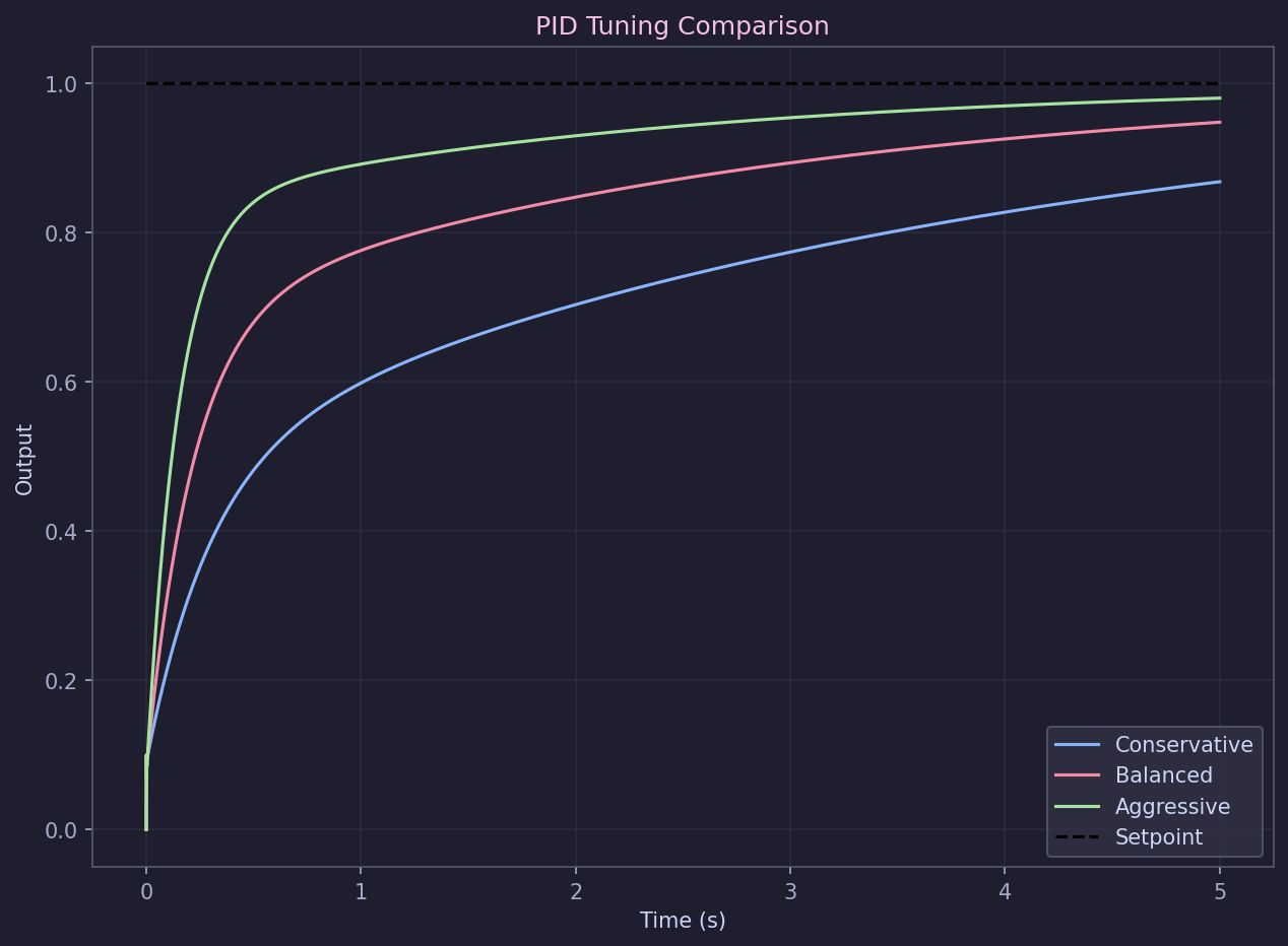
step() simulates the system's response to a unit step input, and stepinfo() extracts the key performance metrics - rise time, overshoot, and settling time. For the thermal chamber application, you want fast rise time to reach setpoint quickly, with minimal overshoot to stay within the 0.5-degree tolerance band.
Stability margins
margin(C*G) plots the Bode diagram of the open-loop transfer function with gain margin and phase margin annotations overlaid. Your targets here are a gain margin greater than 6 dB and a phase margin greater than 45 degrees - these give the system enough robustness to handle modeling errors and component variations without going unstable.
Auto-tuning for comparison
pidtune(G, 'pid') uses numerical optimization to find PID gains that balance performance and robustness automatically. By overlaying both the manual and auto-tuned step responses on the same plot, you can see exactly where your hand-tuned gains trade off differently - maybe faster rise time but more overshoot, or vice versa.
What Just Happened
You went from a plant model to a fully tuned controller with stability margins verified - in under 15 lines of code. The step response, Bode diagram, and performance metrics are all visible immediately in Forge, giving you a complete picture of your control system's behavior without switching between tools or writing boilerplate.
Going Further
- State-space models: Use
ss(),tf2ss(), andss2tf()for MIMO systems, LQR optimal control, and observer design. - Root locus and Nyquist: Use
rlocus()andnyquist()for analyzing systems with more complex dynamics. - Discrete-time: Use
c2d()to convert your continuous controller to discrete-time for microcontroller or PLC implementation.