You have an accelerometer bolted to a test rig and the data is buried in high-frequency noise. Before you can run your vibration analysis, you need a clean signal. In Forge, you can design, verify, and apply a production-quality digital filter in exactly 5 lines.
The 5 Lines
Fs = 1000— set the sample rate[b, a] = butter(4, 100/(Fs/2))— design the filterfreqz(b, a, 1024, Fs)— visualize the frequency responsey_clean = filtfilt(b, a, y_noisy)— apply zero-phase filteringplot(t, y_noisy, t, y_clean)— compare before and after
Walkthrough
Line 1 — Set the sample rate
Fs = 1000 defines the sampling frequency in Hz. Set this to match your data acquisition hardware — here, the accelerometer samples at 1 kHz.
Line 2 — Design the filter
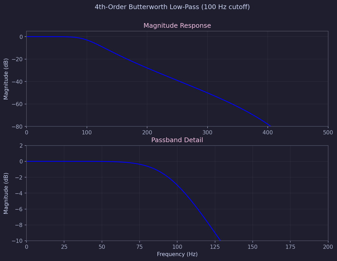
butter(4, 100/(Fs/2)) returns the numerator and denominator coefficients of a 4th-order Butterworth IIR filter. The normalized cutoff is 100/500 = 0.2, giving a maximally flat passband with 80 dB/decade rolloff.
Line 3 — Visualize frequency response
freqz(b, a, 1024, Fs) computes and plots magnitude and phase response over 1024 points. Use this to verify the -3 dB point sits at 100 Hz and stopband attenuation meets your requirements.
Line 4 — Apply the filter
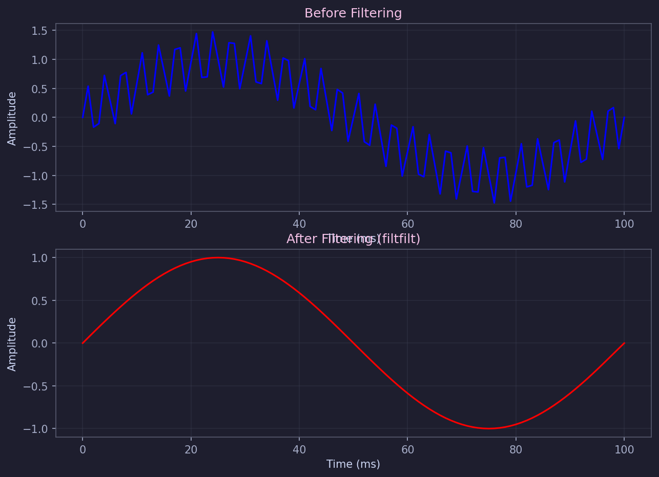
filtfilt(b, a, y_noisy) applies the filter forward then backward, eliminating phase distortion entirely. Peaks and zero-crossings stay exactly where they are — unlike filter(), which would shift the output in time.
Line 5 — Compare results
plot(t, y_noisy, t, y_clean) overlays the noisy and filtered signals so you can visually confirm performance before moving on to analysis.
What Just Happened
In 5 lines, you designed a production-quality digital filter, verified its frequency response, applied it with zero phase distortion, and visualized the results. No imports, no boilerplate, no library installation.
Going Further
- Spectral analysis:
fft(),pwelch(),spectrogram()for time and frequency domain analysis - Peak detection:
findpeaks()with configurable prominence, distance, and threshold - Advanced filter design:
cheby1(),cheby2(),ellip(),fir1(),designfilt()